Notebook Writing Guide
As you are creating notebooks to execute within Losant, this guide provides all the best practices you need to consider when building.
Notebook Process
Before notebooks, to perform some sort of complex batch processing using the IoT data you've collected in Losant, you would have had to figure out how to export all of the data from Losant, perform the processing on your local machine, then upload the result back to Losant (most likely by uploading a CSV to a Data Table).
We've made this much easier with Notebook. Let's look at what this process would be now:
- Configure Inputs - You need to tell Losant what data you need in the Jupyter Notebook for your batch processing.
- Request a Data Export - To test your notebook locally, we need to pull test data from Losant.
- Build Notebook Locally - Write your Jupyter Notebook. This guide will cover tips on how to do this.
- Configure Outputs - You need to tell Losant what output to look for from your notebook.
- Execute Notebook - Let the magic happen within Losant.
This is a really helpful model to keep in mind as you're building your notebooks.
Developing Locally
When we say "Develop Locally" what we mean is that you will need to build a Jupyter Notebook on your computer. Jupyter gives you the ability to export notebooks; this export is what you'll be uploading to Losant as a Notebook File.
Let's walk through a simple example.
Installing Jupyter
If you don't have Jupyter on your machine, you'll need to install it. We strongly recommend installing Python and Jupyter using the Anaconda Distribution, which includes Python, the Jupyter Notebook, and other commonly used packages for scientific computing and data science. When running your notebook with Losant's infrastructure, we use an Anaconda-based environment.
If you prefer to install manually, see the Jupyter Documentation.
Creating a Notebook
Now, let's create a notebook within Losant. In the secondary menu, within an application, select "Notebooks". Then, in the top-right, you'll see an "Add Notebook" button:
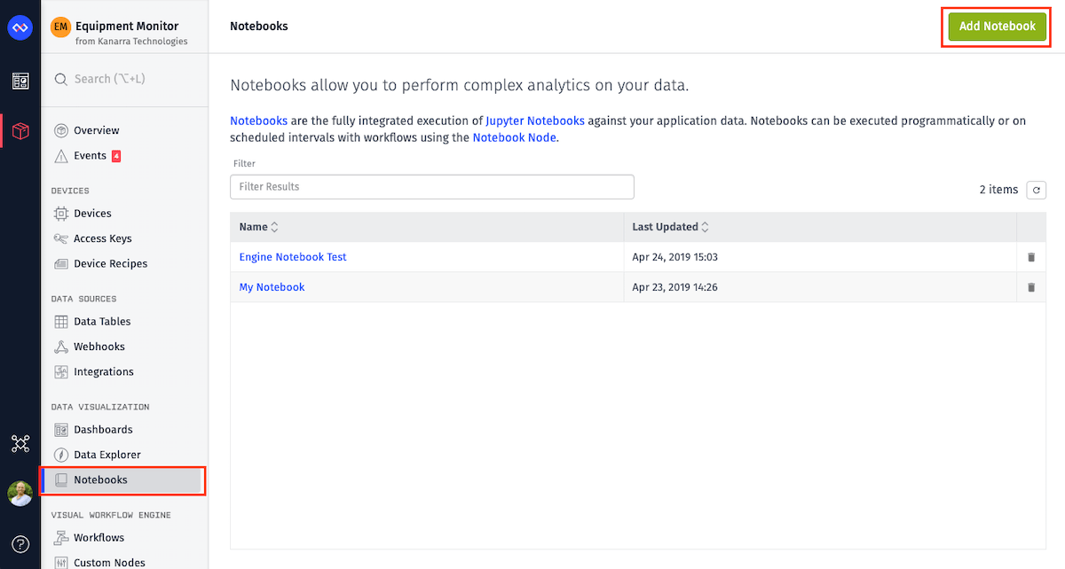
Once here, we can name and describe our notebook. Keep in mind that descriptions are important to give context to unfamiliar team members.
Configure Inputs
As step one of the Notebook Process, we need to configure our inputs. To figure out what inputs you need, you can ask yourself one question: What data or datasets are needed to answer my processing?
For example, if we wanted to analyze the history of engine temperature data and build a complex visualization around that to use in the dashboard, we will need the device data for the engine(s) we would like to analyze.
In your newly created notebook, we can easily configure that as an input.
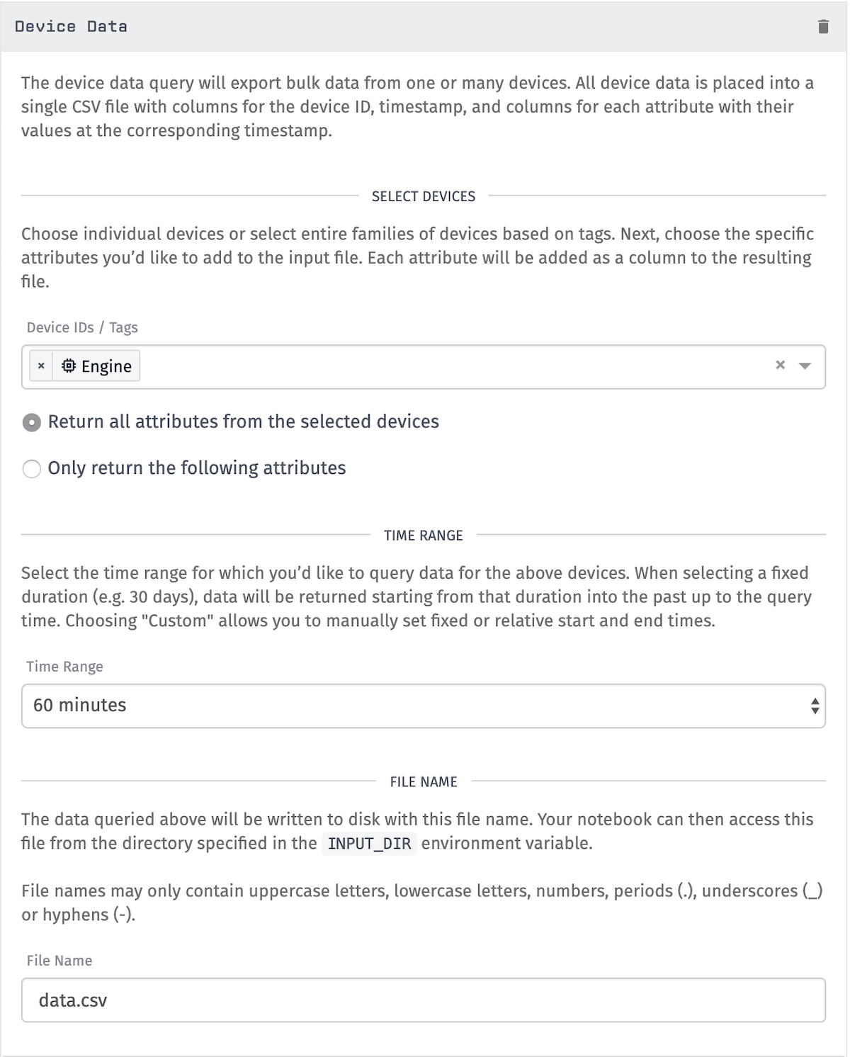
In the settings above, I'm selecting my device Engine, specifying that we want the last 60 minutes of data, and we would like it in a filed called data.csv.
Note: Here, I'm specifying 60 minutes for the sake of a simple example, but notebooks have the ability to pull all the data you have within Losant. You can perform your batch processing over very large datasets.
This "File Name" is important. Since we are naming it data.csv, in the notebook within the INPUT_DIR we should expect to see a file called data.csv.
Request a Data Export
Now that we have identified our dataset and set up the notebook inputs, we need to request a data export.
Before you can even upload a notebook to Losant, you need to create the Jupyter Notebook that performs the desired analysis. Requesting a data exports ensures that, once you upload the notebook to Losant, the format of the data you build your notebook with is the same format that Losant will use to execute the notebook.

Now, you need to configure a Query Time. The Query time is the anchor point against which any device data datasets are built. For example, above we chose the last 60 minutes of data. Normally, this type of query assumes, 60 minutes from now. But, with notebooks it's the last 60 minutes of data from the Query Time. This allows for extremely granular control over what data Losant provides to your notebooks.
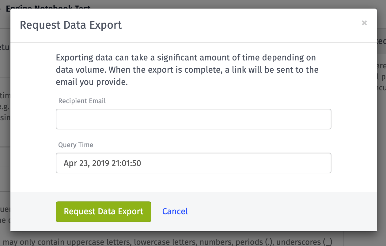
If I chose a Query Time of Apr 10, 2019 12:00:00, and requested the last 60 minutes of data, I'll get all of the device data between the times of Apr 10, 2019 11:00:00 and Apr 10, 2019 12:00:00.
Saving the Inputs
When executing your notebook within Losant we provide the INPUT_DIR and OUTPUT_DIR environment variables. From within the notebook, you'll read these to know where your inputs are and where the outputs should go.
To reproduce this model locally, here is how I structured my folders:
.
└── analytics
  ├── inputs
  ├── outputs
  └── analytics.ipynb
Since we will be running locally, after you receive your data export, save it to your local inputs directory. In my file structure above, I would place data.csv in ~/src/analytics/inputs.
Running a Local Notebook
Depending on how you installed Jupyter, how you run it may be different. If you used the recommended installation above, you should be able to run with:
$ jupyter notebook
Here is how we would run the notebook locally to provide environment variables:
$ cd ~/src/analytics # go to my project folder

# set input and output env vars when running jupyter
$ INPUT_DIR=~/src/analytics/inputs OUTPUT_DIR=~/src/analytics/outputs jupyter notebook
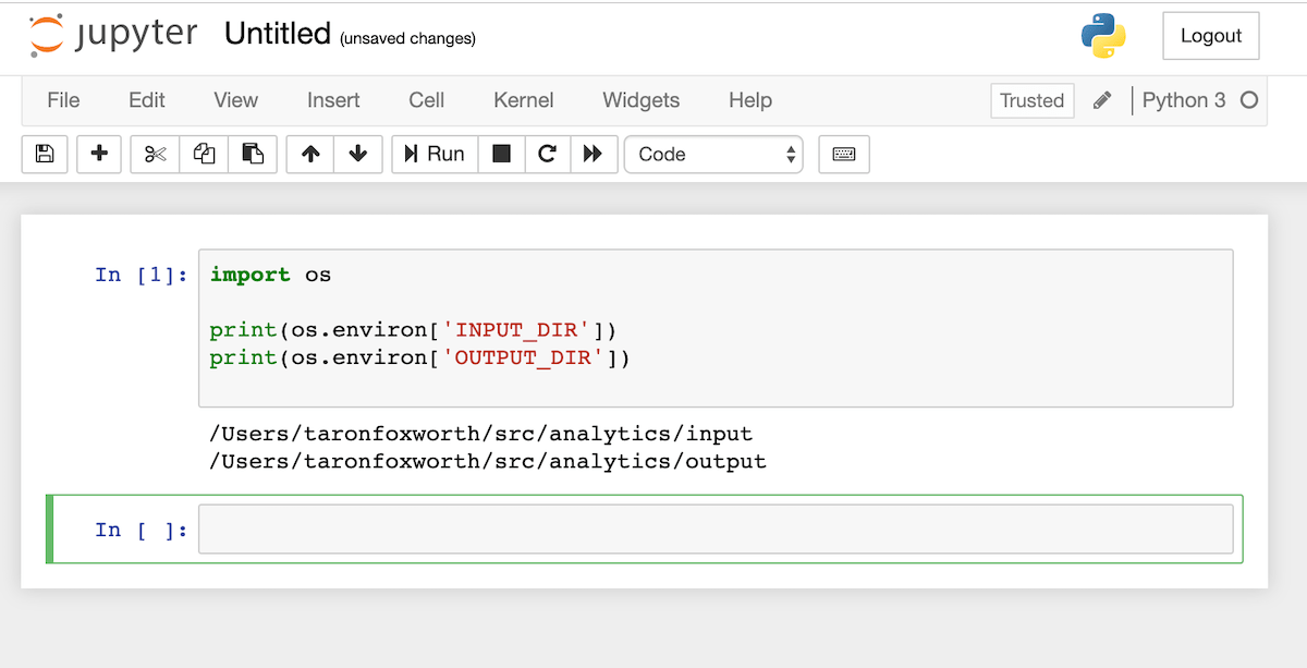
After running the command above, Jupyter should automatically open up in a new browser window:
Building the Notebook
At this point, we have Jupyter installed and our input data within the inputs directory, we are ready to start building the notebook.
Checking Environment Variables
The first thing you should do in your notebook is make sure that you are reading the input and output environment variables correctly:

This simply double checks that the environment variables were read properly.
Notebook Analysis
From here, we can start to build our notebook logic. Every batch processing problem starts with a good question. In your notebook, the goal is to answer your desired question using the input data and derive an output.
In the example above, I wanted to analyze the history of the temperature data for my engine, and build a complex visualization around that to use in the dashboard. Here is an example notebook that does that:
gist:LosantGists/05f1c5eccfc10bc9d2a1c8767d299615
In this notebook, I am taking the Engine temperature data, plotting a histogram, and saving that histogram to a file.
Notebook Explanation
There are some key items to note in the example notebook. First, let's take a look at reading inputs:
data = pd.read_csv(os.path.join(os.environ['INPUT_DIR'], 'data.csv'))

data['Timestamp'] = pd.to_datetime(data['Timestamp'], unit='ms')
data.set_index('Timestamp', inplace=True)
We are reading our data.csv from the input environment variable. For now, this is all local but once you upload your notebook to Losant, Losant will configure the environment variables and file locations for you. On top if that, it will place all of your inputs in the proper spot and the exact same format as the data export.
Next, let's look at the outputs:
## Save Histogram
fig = histogram.get_figure()

output_path = os.path.join(os.environ['OUTPUT_DIR'], 'histogram.png')
fig.savefig(output_path)
We are saving a file called histogram.png in the proper output directory. In general, your notebook can output files and data. Here, in this example, we are simply going to output a file to be saved in Application Files. Later, we will have to configure this output within Losant.
Export Notebook and Upload
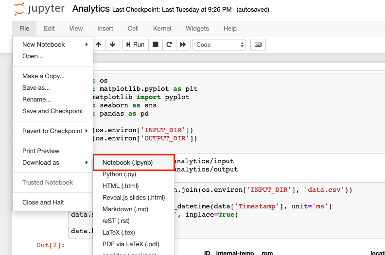
We are ready to export our notebook and upload to Losant for Execution. To export your notebook, go to File > Download as > Notebook (.ipynb) within the Jupyter Application.
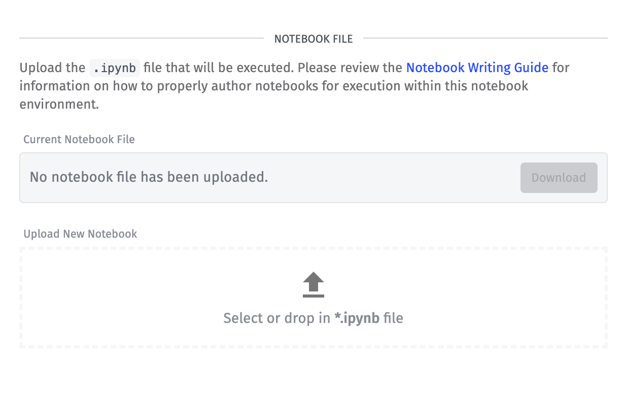
Then, in the "Notebook File" tab of your notebook setting within Losant, you can upload the .ipynb file.
Configuring Outputs
In the notebook we created, we are saving a file called histogram.png in the output directory. In order for Losant to know what to do with the outputs, we will have to configure it.
In the "Outputs" tab of the notebook page, you can add a new Custom File Output.
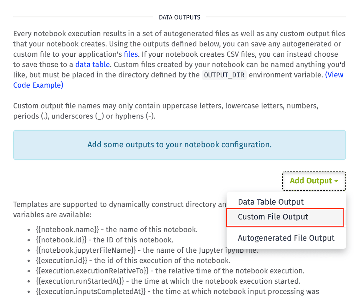
Since we gave it a specific name, we'll have to configure that:
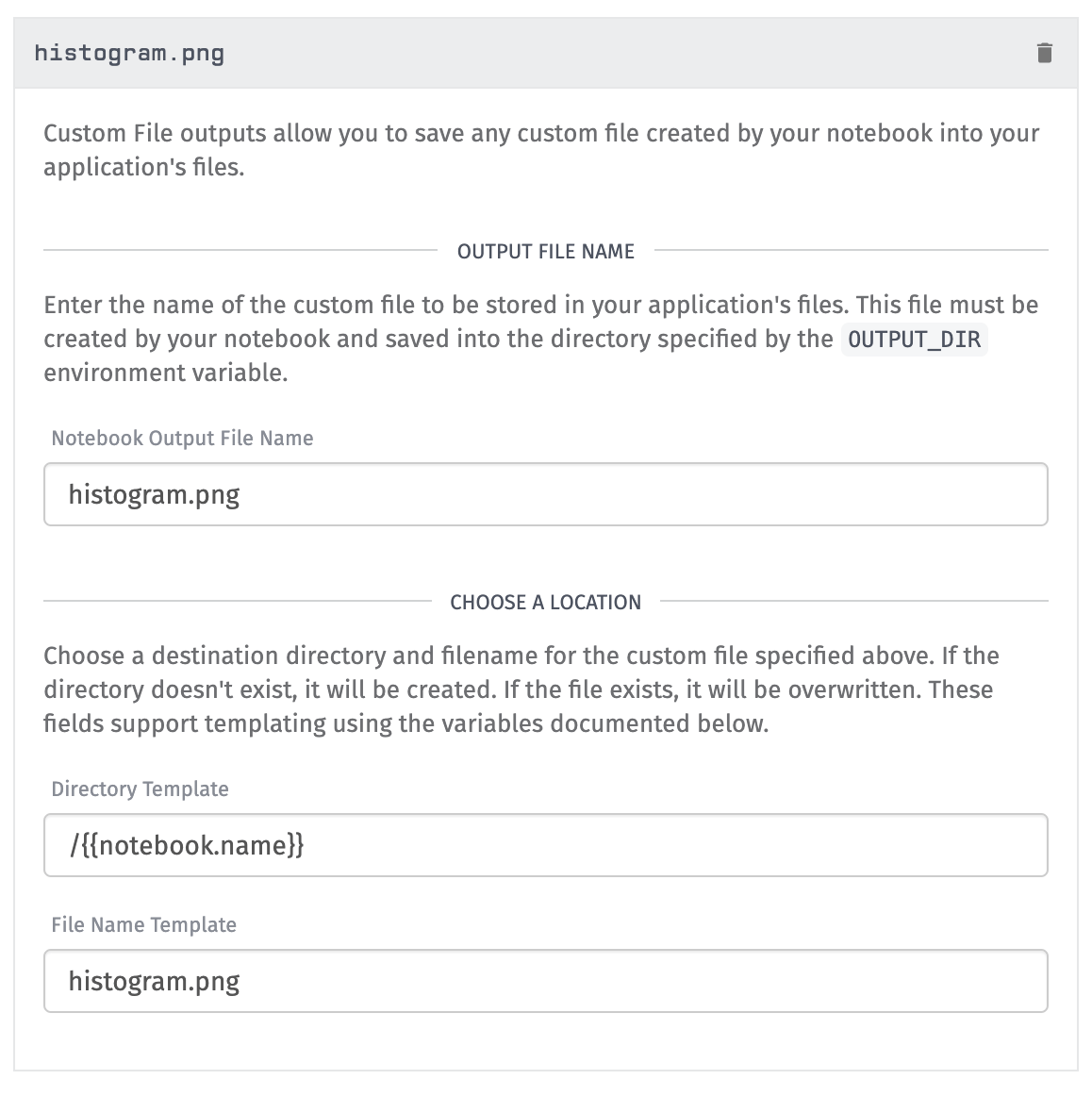
In this config, the "Output Files Name" tells Losant what to look for in your OUTPUT_DIR.
Since this is a Custom File Output, Losant will move this file from your notebook execution environment to Application Files. In the "Choose A Location" settings, you are defining where to put the output within Application Files. Here, we can be really smart about where the file gets saved with templates. In the settings above, we are using the {{notebook.name}} template to save the image in a directory named after the notebook.
Note: This configuration will save over the last histogram.png every time the notebook is executed. This technique is useful if this image is displayed in a Dashboard Block. Because it will get refreshed, the block will stay up to date with the latest results.
Now, let's save the outputs and move on to executing it with Losant!
Execution
We are finally at the last step of the Notebook Process. It is time to execute the notebook. On the main notebook page, in the top-right, you should see the execute button. Once pressed, you'll see the following dialog:
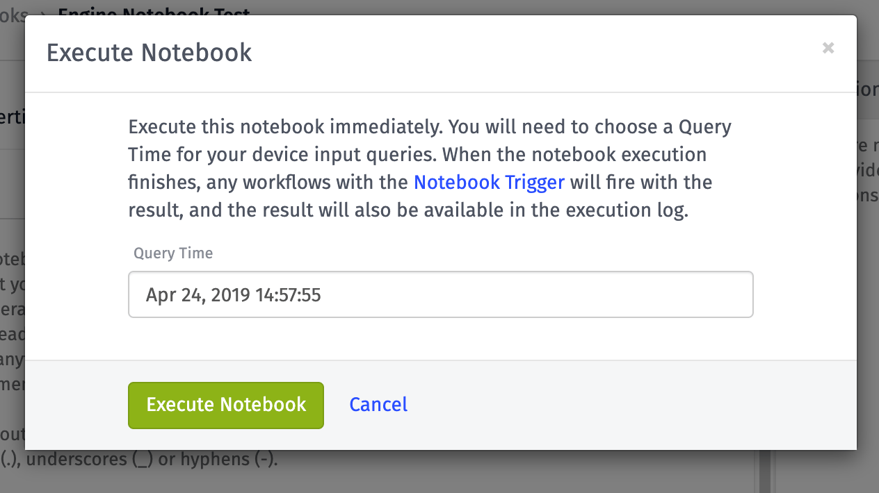
Just as we did for the data export, here we need to define a Query Time and select "Execute Notebook".
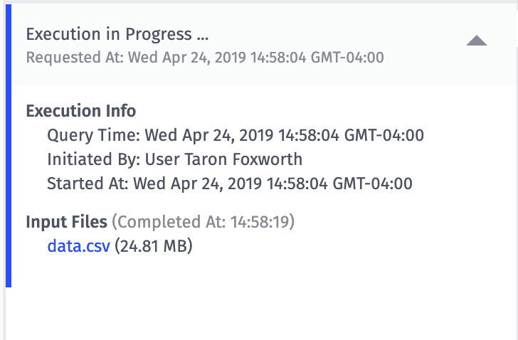
After selected, keep in mind that your notebook won't immediately execute, it will be placed in a queue. To keep you up to date around what's happening with your notebook, Losant provides an Execution Log. Unlike the other logs, this log is persistent.
When your notebook starts executing, you'll see an "Execution in Progress" message:
Once the execution is finished, you'll see an "Execution Completed" message:
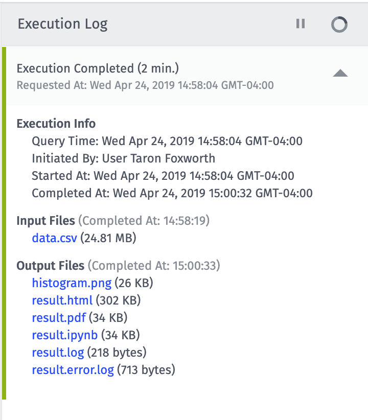
In the log message, you'll be able to see a ton of information about this notebook execution like when it started, and what triggered it.
For your convenience, we also autogenerated some outputs for you, like a PDF version of the notebook execution. These can be really helpful for debugging. Best of all, they can be save to Application Files as an output.
If your notebook execution ends in an error, we have documented all of the possibilities and provided suggestions for how to troubleshoot the issue.
If all was successful, we can find our histogram.png in our Application Files:
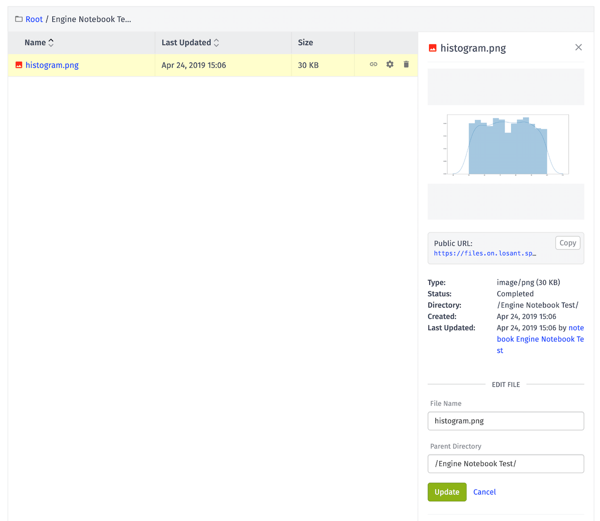
For more detail and background around notebook execution, please refer to the Execution Overview.
Dashboard
Notebooks really become valuable when you integrate the results back into the rest of your Losant application.
In this example, since we created a visualization, it makes a lot of sense to show it on a Losant Dashboard. Since our output image (histogram.png) lives in Application Files, we can easily do this with an Image Block.
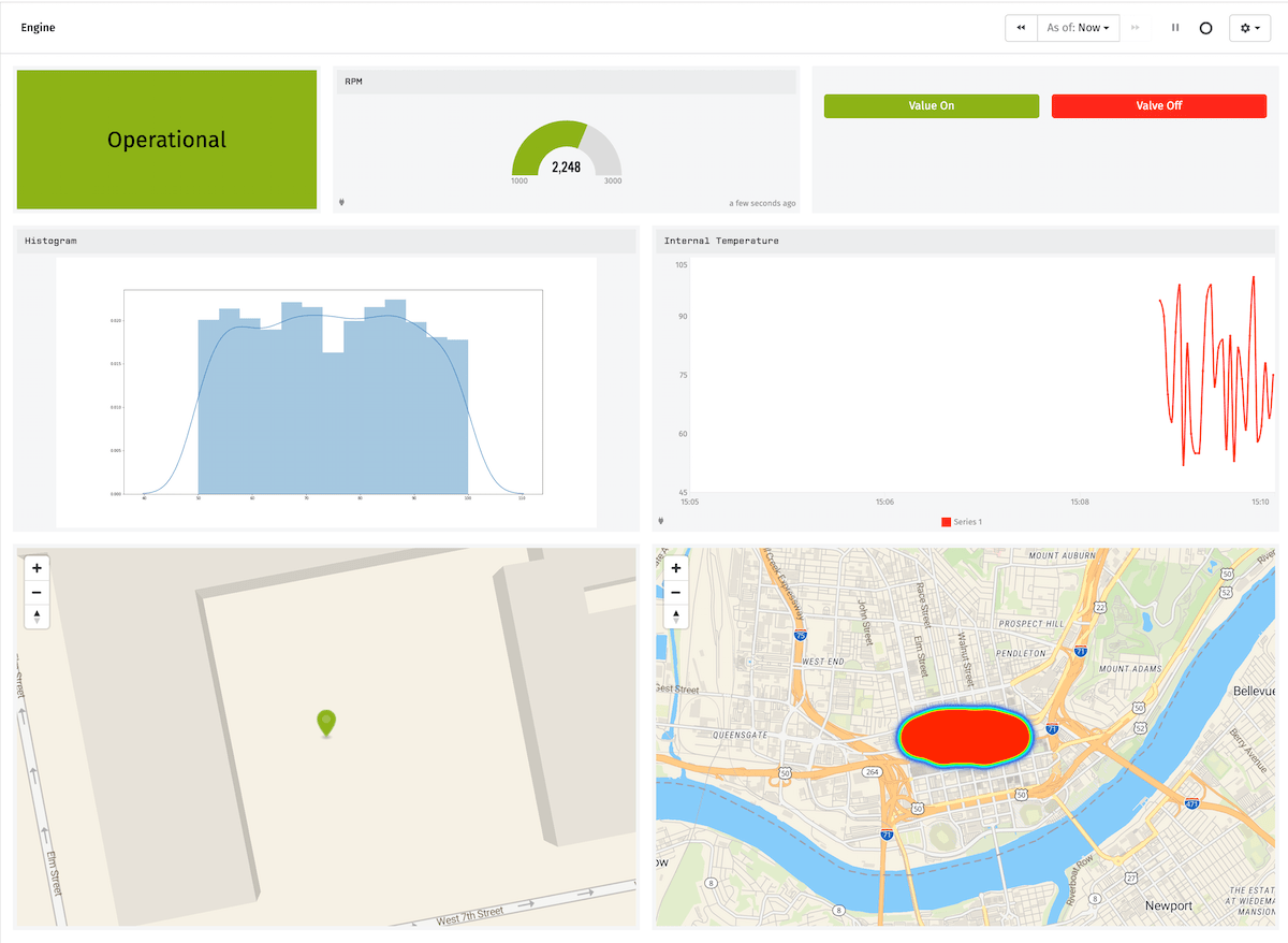
On the other hand, the output of a notebook can be data that results in a Data Table entry. This data can be shown on a dashboard, used to make decisions in a Losant Workflow, or used to power an Losant Experience.
What's Next?
It's time for you to build more complex notebooks. With notebooks, you can answer some really deep and complex questions about your data. By looking at your data over time, what can you learn?
More Resources:
- Notebook Resources - Not familiar with Jupyter Notebooks or Python? We put together some resources that can help.
- Notebook Snippets - Snippets are re-usable source code you can use in your notebooks.
Was this page helpful?
Still looking for help? You can also search the Losant Forums or submit your question there.